- Prerequisites and installing
- Overview of splicing analysis
- Getting annotation together
- Quantifying junctions
- Generating a curated cross-sample junction set
- Comparing junctions
- Overview of splicing analysis
- Quantifying events
- Comparing events
- Sample code for complete analysis
- Simulations
- Building models
- Simulating transcripts
- Comparing events
- Utilities and extras
- quickjunc
- annotate_junctions
- Notes on junction ids
Manual
Prerequisites and installing
Prerequisites
The ENTHOUGHT python distribution (http://enthought.com/products/epd.php) is recommended, if you have troubles getting numpy and scipy installed together.
Spanki requires the following python packages (Python will attempt to install them for you):
Programs required for all functions:
Installing
Clone the repository for most recent changes:
git clone https://github.com/dsturg/Spanki.git
Checkout the branch for the most recent stable release, eg:
git checkout release-0.4.3
Or download the most recent stable release.
Install using the python setup script:
sudo python setup.py install
Overview of splicing analysis
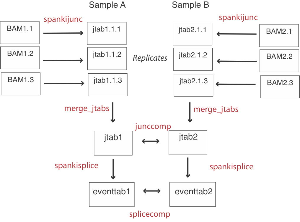
The basic flow of an analysis involves quantifying junctions for each replicate, and then merging the junction results (jtabs) by sample. Then events are quantified using these pooled junction results, and inferences are made by comparing at the junction level and the event level (See flowchart above).
Getting annotation together
Transcript models
Spanki requires an annotation in GTF format for most functions. The annotations from Ensembl are compatible. A slightly altered version of the Drosophila Ensembl annotation is available here: Drosophila Ensembl release 67 (edited)Splicing definitions
Spanki uses splicing definitions generated from the standalone version of AStalavista (Michael Sammeth). http://genome.crg.es/astalavista/Spanki is designed to use pairwise defined events, and is inclusive of alternative first and last exons. To get events defined this way, run AStalavista (versions < 3.0) like this:
./bin/astalavista.sh -c asta -k 2 -i ~/data/annotation/dmel_BDGP5.39.67_ed.gtf -o dmel_BDGP5.39.67_ed.events +ext ;The precomputed splicing events generated as above for Drosophila are here: dmel_BDGP5.39.67_ed.events
More recent versions of the AStalavista software are available here: http://sammeth.net/confluence/display/ASTA/Home. A page describing the new version is here. To define events using the newer version (v 3.2), run it like this:
./bin/astalavista -t asta -i dmel_BDGP5.70_ed.gtf -e [ASE,ASI] ;The output of either AStalavista version is compatible with Spanki.
Junction alignment evaluation
Spanki takes an alignment file in BAM format as input and calculates a variety of confidence metrics about spliced alignments. The BAM file can be from any aligner, but has only been tested on BAM files produced by Tophat (Trapnell et. al, http://tophat.cbcb.umd.edu)Usage:
spankijunc -i alignments.bam -g genemodels.gtf -f genome.fa [Options]
| Options: | |
| -i <string> | input alignments (required) |
| -o <string> | output directory [default: junctions_out] |
| -g <string> | reference gtf (required) |
| -f <string> | reference fasta (required) |
| -m <string> | analysis mode (see below): all, eval, quant [Default: all] |
| -filter <string> | T,F [Default: F (report all alignments)] |
| -r <int> | Size to examine for repeats (number of bases, default=10) |
| -ohang <int> | Overhang applied to junction filtering and intron retention analysis (number of bases, default=8) |
Analysis modes:
Spanki offers three bundles of analyses to perform. The "quant" mode performs quantitation only, and the "eval" mode generates more quality criteria to help evaluate the validity of the junction. The "all" default mode performs all available analyses. ThFields reported:
unfilt_cov:	Junction coverage including small anchors
cov:		Junction coverage where minimum anchor size is >= 8
normcov:	Coverage normalized by sequencing depth (divided by million mapped reads)
annostatus:	A code for the annotation status of the join
	* an = annotated
	* un.ad = unannotated join, annotated donor
	* un.aa = unannotated join, annotated acceptor
	* un.ad.ad = unannotated join of annotated donor and acceptor
geneassignL:	Gene assignment of "Left" edge
geneassignR:	Gene assignment of "Right" edge
geneassign:	Gene assignment of entire join
gmcode:	A code for the gene model where this join resides.  Code is "num transcripts.num introns.num starts"
 eg:      3t.21i.3s  A gene with 3 transcripts, 21 introns, and 3 start sites
regcode:  A code for the type of regulation annotated in the gene model
	* ap = alternative promoters
	* as = alternative splicing
	* asap = alternative promoters and splicing
	* con = constitutive, multi-exon
	* se = single exon
offsets:	Number of unique starting positions for junction alignments
entropy:	Entropy calculation described in Graveley et al., 2011
hamming3:	Edit distance between the 5-prime intron sequence and the 3-prime exon anchor
hamming5:	Edit distance between the 3-prime intron sequence and the 5-prime exon anchor
dinucleotide:	Donor and acceptor motifs (eg "GT..AG")
MAXmmes:	Maximum of the minimum match on either side for all alignments to this junction (Wang L., et al., 2010)
MAXminanc:	Maximum of the minimum anchor sizes or all alignements to this junction.
lirt:		Intron read-through on the “Left” side
rirt:		Intron read-through on the “Right” side
irt:		Total intron read-through
datrans:	Donor to acceptor transition probability
dncov:		Coverage for all joins connected to this donor
ancov:		Coverage for all joins connected to this acceptor
Filtering:
By default, all junctions are reported, along with criteria for filtering them. This is the preferred approach, so you can apply custom criteria for flitering. You may also turn on automatic filtering to remove junctions that have these characteristics:Merging junction tables
The "merge_jtabs" function pools results together for more than one replicate. Output is written to standard out:Usage:
merge_jtabs rep1/juncs.all,rep2/juncs.all,rep3/juncs.all > sample1_repsmerged.juncs
Generating a curated cross-sample junction set
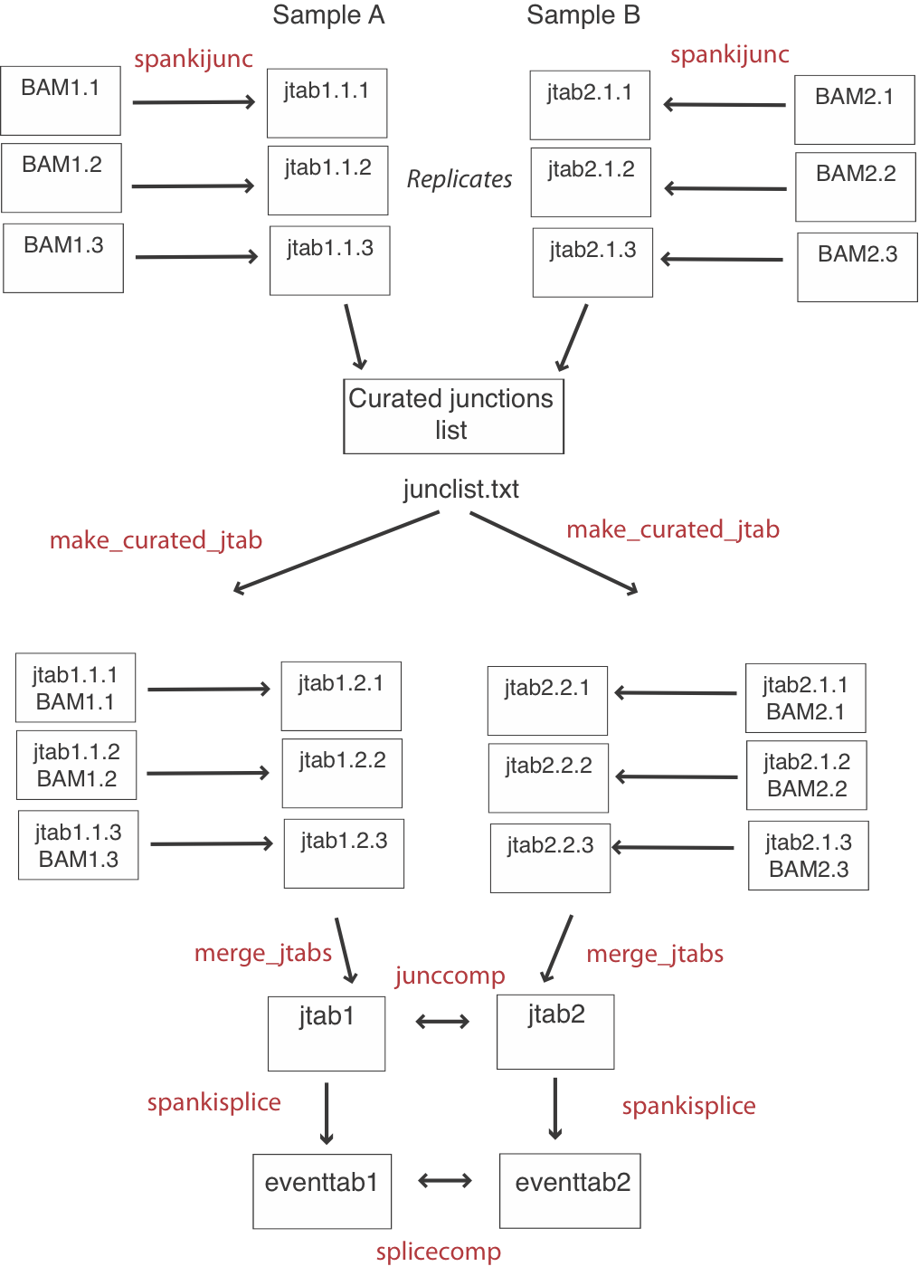
If you are only interested in annotated splicing events, this step is optional. For a detailed junction-level comparison, it is better to do all junction quantification first, then make a list of curated junctions detected in any sample. Then, you can run a cleanup script on each replicate, to calculate intron read-through and donor coverage for junctions that were NOT detected. This will give you symmetrical junction tables with results for the same number of junctions for each replicate (See flow chart above). After making a list of curated junctions, get additional data from each replicate lke this:Usage:
make_curated_jtab -i alignments.bam -jlist oklist.txt -jtab juncs.tab
| Options: | |
| -o <string> | output directory [default: curated_juncs] |
| -i <string> | input alignments (required) |
| -jlist <string> | list of curated junctions |
| -jtab <string> | first pass junction table for this BAM |
| Options: | |
| -a <string> | junction table for sample A (Output of spankijunc) |
| -b <string> | Junction table for sample B (Output of spankijunc) |
| -o <string> | output directory [default: junccomp_out] |
| -g <string> | reference gtf (required) |
Output:
juncid:	Unique junction identifier
geneassign:	Gene assignment of entire join
annostatus:	A code for the annotation status of the join
	* an = annotated
	* un.ad = unannotated join, annotated donor
	* un.aa = unannotated join, annotated acceptor
	* un.ad.ad = unannotated join of annotated donor and acceptor
intron_size:	Length of intron in bp
gmcode:	A code for the gene model where this join resides.  Code is "num transcripts.num introns.num starts"
 eg:      3t.21i.3s  A gene with 3 transcripts, 21 introns, and 3 start sites
regcode:  A code for the type of regulation annotated in the gene model
	* ap = alternative promoters
	* as = alternative splicing
	* asap = alternative promoters and splicing
	* con = constitutive, multi-exon
	* se = single exon
avg_totalcov:	Average of total coverage in both samples
cov1:	Coverage in sample A
irt1:	Intron retention reads in sample A (donor and acceptor side)
dncov1:	Donor neighbor coverage in sample A
donor_irt1:	Intron retention reads over the donor
totalcov1:	Total coverage over donor in sample A (cov1 + dncov1 + donor_irt1)
cov2:	Coverage in sample B
irt2:	Intron retention reads in sample B (donor and acceptor side)
dncov2:	Donor neighbor coverage in sample B
donor_irt2:	Intron retention reads over the donor
totalcov2:	Total coverage over donor in sample B (cov2 + dncov2 + donor_irt2)
PSI_IRT1:	Intron retention in sample A (as "Percent Spliced In")
PSI_IRT2:	Intron retention in sample B (as "Percent Spliced In")
deltaPSI_IRT:	Difference in intron retention between A and B
pval_irt:	P-value for intron retention difference based on Fisher's exact test
qval_irt:	Benjamini-hochberg adjusted p-value
PSI_donor1:	Percent spliced in for this junction relative to other donor coverage
PSI_donor2:	Percent spliced in for this junction relative to other donor coverage
deltaPSI_donor:	Difference in donor PSI
pval_donor:	P-value for donor PSI based on Fisher's exact test
qval_donor:	Benjamini-hochberg adjusted p-value
minp:	Minimum p-value from either significance test
Splicing event analysis
Spanki uses splicing definitions from AStalavista. From this, Spanki extracts junction coverages that define each event, which is partitioned into inclusion and exclusion paths. Comparisons are made using Fisher’s exact tests. This general approach was first developed by Eric Wang and extended by A. Brooks et. al, 2011 (see Refs). The differential splicing testing used is similar to JuncBASE (See http:// compbio.berkeley.edu/proj/juncbase/).See the section "Getting annotated together" if you have not already made your AStalavista splicing definitions.
Quantification of inclusion / exclusion paths
The script "spankisplice" quantifies inclusion/exclusion paths Usage:spankisplice -j juncs.all -c isoform FPKMs -g genemodels.gtf -f genome.fa -a events [options]Example:
spankisplice -o female_repsmerged_events -j female_repsmerged.juncs -c testdata/female_cuff/isoforms.fpkm_tracking -f testdata/fasta/myref.fa -g testdata/annotation/genemodels.gtf -a testdata/annotation/genemodels_splices.out
| Options: | |
| -i <string> | input alignments (required) |
| -o <string> | output directory [default: spankisplice_out] |
| -g <string> | reference gtf (required) |
| -f <string> | reference fasta (required) |
| -jtab <string> | Junction quantifications |
| -a <string> | AStalavista events annotation (required) |
| -c <string> | Cufflinks output (optional) |
| -v <T/F> | Verbose output (default: F) |
| Options: | |
| -a <string> | events table for sample A (Output of spankisplice) |
| -b <string> | events table for sample B (Output of spankisplice) |
| -o <string> | output directory [default: splicecomp_out] |
| -g <string> | reference gtf (required) |
| -cc <int> | coverage cutoff for significance testing (default - no cutoff) |
event_id 	Unique identifier for the event
gene_id	Gene id
gene_name	Gene name
transcript_id	Transcripts with inclusion or exclusion form, separated by a comma
eventcode	A code for the event type
structure	AStalavista structure code
joinstring	Junction ids defining the inclusion or exclusion form
inc_sites	Number of 'sites' (junctions) in inclusion path
exc_sites	Number of 'sites' (junctions) in exclusion path
inc1	Inclusion coverage, sample A
exc1	Exclusion coverage, sample A
psi1	PSI, sample A
inc2	Inclusion coverage, sample B
exc2	Exclusion coverage, sample B
psi2	PSI, sample B
delta_psi	Delta PSI
totalcovpersite1	Total coverage per site in sample A
totalcovpersite2	Total coverage per site in sample B
avgcovpersite	Average coverage per site
pval	P-value for donor PSI based on Fisher's exact test
qval	Benjamini-hochberg adjusted p-value
fpkm_proportion1	FPKM proportion, sample A (if abundances supplied)
fpkm_proportion2	FPKM proportion, sample B (if abundances supplied)
Complete pipeline:
A pipeline with a sample run is in the file analysis_commands.sh. Make a working directory somewhere, and decompress the test data from there: testdata.tar.gz Also copy analysis_commands.sh to this directory and run it. It will run the following commands:echo "[***************] Starting female spankijunc runs" spankijunc -m all -o female_rep1 -i testdata/female_r1.bam -g testdata/annotation/genemodels.gtf -f testdata/fasta/myref.fa spankijunc -m all -o female_rep2 -i testdata/female_r2.bam -g testdata/annotation/genemodels.gtf -f testdata/fasta/myref.fa echo "[***************] Starting male spankijunc runs" spankijunc -m all -o male_rep1 -i testdata/male_r1.bam -g testdata/annotation/genemodels.gtf -f testdata/fasta/myref.fa spankijunc -m all -o male_rep2 -i testdata/male_r2.bam -g testdata/annotation/genemodels.gtf -f testdata/fasta/myref.fa echo "[***************] Merging the replicates together" merge_jtabs female_rep1/juncs.all,female_rep2/juncs.all > female_repsmerged.juncs merge_jtabs male_rep1/juncs.all,male_rep2/juncs.all > male_repsmerged.juncs echo "[***************] Parsing events output" spankisplice -o female_repsmerged_events -j female_repsmerged.juncs -c testdata/female_cuff/isoforms.fpkm_tracking -f testdata/fasta/myref.fa -g testdata/annotation/genemodels.gtf -a testdata/annotation/genemodels_splices.out spankisplice -o male_repsmerged_events -j male_repsmerged.juncs -c testdata/male_cuff/isoforms.fpkm_tracking -f testdata/fasta/myref.fa -g testdata/annotation/genemodels.gtf -a testdata/annotation/genemodels_splices.out echo "[***************] Doing pairwise comparison" splicecomp -a female_repsmerged_events/events.out -b male_repsmerged_events/events.out -o F_vs_M_splicecomp junccomp -a female_repsmerged.juncs -b male_repsmerged.juncs -o F_vs_M_junccomp
Simulations
Overview
Below is a basic guide to running simulations with Spanki. It uses the test dataset avaliable at: http://www.cbcb.umd.edu/software/spanki/testdata.tar.gzRetrieve and decompress testdata.tar.gz in a working directory, and run the example commands below to try it out.
To see example simulated data, see here:
Getting started
Spanki's simulator has several options to incorporate errors into simulated reads. Custom models are an option that uses models generated from permissive Bowtie mapping. To build custom models, Spanki requires Bowtie alignments in map format. If you don't wish to build custom models, you can jump straight to "Simulating transcripts"Building custom models (optional)
The program 'spankisim_models' will make error models from a Bowtie map file. See http://bowtie.cbcb.umd.edu for information about making Bowtie map files. Here is an example of a command for a basic quality-aware Bowtie run:bowtie -p 8 -m 1 --solexa1.3-quals dm3 -1 R63s_5_1_sequence.txt -2 R63s_5_2_sequence.txt R63L5_dm3.mapNote that spankisim_models is a standalone perl script. It doesn't require any external libraries, so it's possible to send it to a cluster to run separately.
Here is how to generate models, using the example map file included in the test dataset. Note that this command does not currently accept aligment file in SAM format (Bowtie2's default output format).
spankisim_models -i testdata/example.map -ends 2 -l 76 -o example_model
| Options: (No defaults) | |
| -o <string> | output directory |
| -i <string> | map file |
| -e <int> | Must be 1 or 2 (single or paired-end) |
| -l <int> | read length |
Simulating transcripts
This will generate simulated reads for every transcript in the provided reference. The number of reads simulated is based on input values of either reads per kilobase (rpk) or coverage (cov). If neither of these is provided, all transcripts are simulated to 1x coverage. Optionally, a text file can be provided that specifies a value for rpk or cov for each transcript. This allows you to build a simulated dataset with heterogeneous transcript abundances.
The simulation can use custom models built from your own RNA-Seq data, or one of several built-in models. Pre-built models include sets built from external controls ("NIST", Jiang et al., 2011), from D. melanogaster whole adult RNA-Seq ("dm3", Graveley et al., 2011), or D. melanogaster head tissue RNA-Seq ("flyheads"). For each of these empirical models, read lengths up to 76bp are supported. The default (random) model works for any read length, and incorporates up to 10 mismatches from a weighted random distribution (with weights [30,20,15,10,5,5,5,5,2.5,2.5]), equal probability of each substitution type, and increasing probablity of mismatch with increasing base position. Error-free reads can also be produced, that have no mismatches relative to the reference
Usage:
sim_transcripts -g genemodels.gtf -f genome.fa [options]Example: using a pre-built model ('flyheads',from an RNA-SEQ experiment on Drosophila heads)
spankisim_transcripts -o sim_flyheads -g testdata/annotation/genemodels.gtf -f testdata/fasta/myref.fa -bp 76 -m flyheads -cov 5 -ends 2Here is an example of using the custom model, from the "Building models" example above:
spankisim_transcripts -o sim_custom -g testdata/annotation/genemodels.gtf -f testdata/fasta/myref.fa -bp 76 -m custom -mdir example_model -cov 5 -ends 2
| Options: | |
| -o <string> | output directory [default: sims_out] |
| -g <string> | reference gtf (required) |
| -f <string> | reference fasta (required) |
| -bp <int> | read length [default: 76] |
| -cov <int> | coverage to simulate [Deafult: if nothing specified, coverage=1 for all transcripts] |
| -rpk <int> | reads per kilobase (rpk) to simulate |
| -ir <float> | intron retention to simulate (range from 0 to 1) [default 0] |
| -m <string> | mismatch model ['random' (default),'errorfree', 'NIST','dm3','flyheads', or 'custom'] |
| -mdir <string> | custom model directory (only needed if you use 'custom' as the mismatch model) |
| -ends <int> | Number of mates (1=single or 2=paired ends) |
| -frag <int> | fragment size [default 200] |
| -t <string> | transcript coverages file (details below) |
Optional transcript file:
A text file of transcripts and abundances to simulate can be supplied separately. This is essential if you only want to simulate a few transcripts, or to simulate different proportions. This file has two columns: transcript ids and either coverages or RPK. Column headers must be present
Example:
txid       rpk
FBtr0081760	100
FBtr0081761	100
FBtr0081759	200
or:
txid       cov
FBtr0081760	5
FBtr0081761	5
FBtr0081759	10
Utilities and extras
quickjunc - Quick junction coverage calculator
Quantifies only junction coverages, evaluates only anchor size Example:quickjunc -i alignments.bam -a 8Options:
-i  Input alignments
-a  Anchor size		[Default=8]
Junction annotator
"annotate_junctions"Takes as input a set of junctions - either a list of junctions, or a table with junctions and other data (such as the 'juncs.all' file from spankijunc). User must also specify a reference genome, and may also include an annotation in GTF format (optional). Alternatively, you can input only the annotation, and the script will analyze all annotated junctions
Output includes qualitative information about each junction. This includes gene assignments and gene model codes (See above: Junction alignment evaluation. In addition, sequence surrounding the junction is output:
juncid	flank5	intron5	intron3	flank3
chr2L:10001434_10002187:-	TACATCCAATTCCGATTCGA	GTGAGTAGATTCCAAGTGAT	CCCATCCATTACAAACGTAG	AAAATATGGAACACCAACTG
chr2L:10002238_10002296:-	GATTGAAGACCCTTAACTTG	GTATATTATTGTAAACATAA	CTATTAAAATATCTTTGCAG	CTGTTCAACTGAGGCGATGT
chr2L:10002343_10002398:-	ACGTAGGATTTTAGTAATAT	GTATTTATTTCTAACTAAAA	ACATTTGATTTGACTTTCAG	AAAATATTGGACTGGATTGC
chr2L:10002343_10002405:-	AGTTGGAACGTAGGATTTTA	GTAATATGTATTTATTTCTA	ACATTTGATTTGACTTTCAG	AAAATATTGGACTGGATTGC
This includes 20bp (sense strand) five-prime exonic flanking sequence (flank5), five-prime intronic sequence (intron5), three-prime intronic sequence (intron3), and three-prime exonic flanking sequence (flank3).
An analysis of NAG motifs is also performed:
juncid	nag	nagframe	nag0	nag3	nag6	totalframenag
chr3R:991557_991801:+	6	6	-	-	chr3R:991557_991810:+	1
For each junction, nag motifs are search for in a nine-codon window. The 'nag' field includes the positions of all nags found. The 'nagframe' field specifies the position of all in-frame nags. Junction ids for all nags found in the three-prime exonic region are given.
Here is an illustration for how NAG positions are numbered:

Examples:
# Annotating a junction set (From a junction table)
annotate_junctions -o female_rep1_annotated_junctab -jtab female_rep1/juncs.all -f ~/data/indexes/dm3_NISTnoUextra.fa -g ~/data/annotation/dmel_BDGP5.39.67_ed.gtf# Annotating a junction set (From a junction list)
annotate_junctions -o female_rep1_annotated_junclist -jlist female_rep1/juncs.list -f ~/data/indexes/dm3_NISTnoUextra.fa -g ~/data/annotation/dmel_BDGP5.39.67_ed.gtf# Annotating annotated junctions
annotate_junctions -o annotated_reference_juncs -f ~/data/indexes/dm3_NISTnoUextra.fa -g ~/data/annotation/dmel_BDGP5.39.67_ed.gtf
Notes on junction identifiers
The junction ID used by spanki is the position of first base of the intron on "left" side (donor site "G" if plus, acceptor site "C" if minus) and position of last base in intron on "right" side (acceptor "G" if plus, donor "C" if minus) in 1-based coordinates (and inclusive). The lower coordinate number is always given first. The coordinates are separated by an underscore, with the chromosome at the beginning and the strand at the end, separated by colons.Example:
chr2R:5702257_5702656:+
Here is an example of a minus strand junction
chr2R
012345678
NNCTNACNN
123456789
(So, chr2R:3_7:- in example above)
Here is an example of a plus strand junction
012345678
NNGCNATNN
123456789
(So, chr2R:3_7:+ in example above)