
Training Manual
Introduction
This manual describes the procedures for training the ab initio
eukaryotic gene finder TigrScan. This
should be done whenever the gene finder is to be applied to a new
organism.
TigrScan is both retrainable and
reconfigurable. The types of
models used
by the program to identify specific classes of gene features can be
specified during training, so that, for example, donor sites might be
detected by weight matrices (WMMs) while acceptor sites might be
detected by 2nd order weight array matrices (WAMs), etc.
Because the different types of models are themselves
parameterizable to varying degrees, it is important during training to
identify the most effective parameters for the chosen set of models.
Obtaining truly optimal performance will, in general, require a
systematic exploration of these multi-dimensional parameter
spaces. This manual describes tools and techniques that can be
used to effectively search those parameter spaces.
Below are the main steps necessary for training
the gene finder:
These steps are described below, followed by a section
of Miscellany.
Step 1. Set environment
variables
Before beginning, please set the following environment variables:
variable
|
value
|
PERLLIB
|
path to perl directory distributed with TigrScan
|
TIGRSCAN
|
path to main installation directory of TigrScan
|
Step 2. Collect training
materials
The training process requires only two files: a
multi-FASTA file of substrate sequences (i.e., contigs or BACs), and a GFF
file
containing the coordinates of coding exons on those substrates.
Each entry in the FASTA file must contain a unique substrate identifier
at the beginning of its defline:
>617264 ...possibly with other
information here...
TACGTAGCTATATTCCGCGATGCTAGCGATTGATCGTA
GCTATATATATCGGCGTCGATGCTAGCTGACTGACTGC
...
This substrate identifier must be the first field in the
GFF records for exons on that substrate:
617264
homo-sapiens initial-exon 1432 1567
. + . transcript_id=1
617264
homo-sapiens internal-exon 1590 1812
. + . transcript_id=1
617264
homo-sapiens final-exon 2276
2571 . + . transcript_id=1
Note that the fields in a GFF record must be separated by tabs
(not spaces), as
stated
in the specification of the GFF standard: <http://www.sanger.ac.uk/Software/formats/GFF/GFF_Spec.shtml>
The fields of the GFF records are:
substrate species exon-type begin end
score strand frame ID
These are explained in detail below:
- substrate : contig or BAC identifier
- species : species or name of program
which generated the GFF, with no whitespace; unused by TigrScan
- exon-type : initial-exon, internal-exon,
final-exon, or single-exon, or exon
- begin: 1-based coordinate of the leftmost
base in the feature, so that a feature beginning at the first base
would have a start coordinate of 1
- end : 1-based coordinate of the rightmost
base in the feature
- score : not necessary, may be a dot (.)
- strand : + or -
- frame : not necessary, may be a dot (.)
- ID : transcript identifier, for grouping
exons into a transcript
Remember that in GFF the begin coodinate is always
less than the end coordinate, even on the reverse strand. Also,
remember that the coordinates are 1-based (so that the very
first base on the substrate has coordinate 1) and are inclusive
(so that the length of a feature is end-begin+1).
Note that your coordinates should include both the start codon and the
stop codon in the transcript sequence. It is common practice, for
example, to give the coordinate of the final coding codon (before the
stop signal) as the end of the final exon, but this will cause the
gene-finder to perform terribly because it will not see the true stop
codon examples during training.
|
IMPORTANT: |
 |
|
Throughout this document we will refer
to coding exons simply as "exons." Currently, the scripts for
generating the training sets for TigrScan do not accept non-coding
exons. If you have example non-coding exons, these can be used to
train the UTR models, but you will have to extract the sample UTRs
yourself until the scripts are modified to accept non-coding exons.
|
Another step which you can perform at this point is to copy some of the
default files from the tigrscan directory into your training
directory. You may modify or overwrite these during training, but
often the defaults are used as-is for the first round of training:
tigrscan.top
|
polya0-100.model
|
train.sh
|
TATA0-100.model
|
single.iso
|
tigrscan.cfg
|
Step 3. Extract training
features
Separating isochores
TigrScan can handle different isochores (ranges of
GC-content) differently. This is generally advantageous, since
exons in different isochores can have different statistical
properties. TigrScan accommodates the differential treatment of
isochores by essentially allowing a separate configuration file and set
of models for each isochore. Thus, the first step in training is
to partition the training set according to isochore, so that the
isochore-specific models can be trained on examples having the proper
GC-content.
A common isochore partitioning for human is:
isochore 1:
|
0% - 43%
|
isochore 2:
|
43% - 51%
|
isochore 3:
|
51% - 57%
|
isochore 4:
|
57% - 100%
|
where the percentages refer to G+C
content, computed as
100*(G+C)/(A+C+G+T) for the given empirically observed nucleotide
counts of a sequence.
If you do not have much training data then you can define a single
isochore covering 0% - 100%.
Once you have decided on a set of isochore boundaries, use the script split-by-isochore.pl
to partition the training data according to GC-content:
split-by-isochore.pl train.gff
contigs.fasta . 4 0 43 51 57 100
where the dot (.) denotes the current directory as the target for the
output files, 4 is the number of isochores being defined, and
0,43,51,57,100 are the isochore boundaries as shown in the table
above.
This script will create a GFF file and a multi-FASTA file for each
isochore (e.g.,
iso0-43.gff and iso0-43.fasta, etc.). It will
also output two files,
gc.txt and bincounts.txt which contain,
respectively, all the GC%
values for all of the transcripts, and a table showing how many
transcripts occurred in each isochore.
Extracting positive examples
The get-examples.pl script is used to
extract the
actual nucleotide sequences for each of the features in the training
set:
get-examples.pl
iso43-57.gff iso43-57.fasta
This command will create the following files:
initial-exons43-57.fasta
final-exons43-57.fasta
internal-exons43-57.fasta
single-exons43-57.fasta
donors43-57.fasta
acceptors43-57.fasta
start-codons43-57.fasta
stop-codons43-57.fasta
introns43-57.fasta
intergenic43-57.fasta
five-prime-UTR43-57.fasta
three-prime-UTR43-57.fasta
Each of these files will later serve as the input to a training
procedure for a specific model of the gene finder. Note that if
you are using only one isochore and you did not use the split-by-isochore.pl
program, you must rename your GFF and FASTA files to iso0-100.gff
and iso0-100.fasta so that the get-examples.pl
program can parse the isochore definition from the filename (in this
case, 0% to 100%).
|
IMPORTANT: |
|
|
Be sure to examine these FASTA files to
ensure that the expected consensus sequences are found at the expected
locations. This will allow you to verify that the coordinates
which you provided for the sample exons were interpreted correctly by
the extraction script. The exon sequences should not contain
start/stop codons nor donors/acceptors at their respective ends, while
the donor/acceptor/start-/stop- codon files should contain the expected
consensus at position 80. You might also verify that no
extraneous characters, such as N's, occur in the extracted example
files. The get-transcripts.pl script in the perl
directory should also prove useful.
|
Extracting negative examples
Once the positive examples have been extracted, a set
of negative examples must be extracted using the get-negative-examples-iso.pl
script. These negative examples are used for evaluating each
model during training so that the parameter space of the model can be
searched. The usage of the command for an individual isochore is:
get-negative-examples-iso.pl
43-57
If you specified an output directory other than "." in the
split-by-isochore.pl command above, then you must first change
into
that directory.
Step 4. Train signal
sensors
Signal sensors are models which are used to detect the
fixed-length features of genes, which include
start codons
|
donor sites
|
stop codons
|
acceptor sites
|
promoters
|
poly-A signals
|
These different feature types will
be referred to as signal
types. For each signal type in each isochore you must train a
model to detect those signals. Each of these models can in turn
be of a different model type.
There are simple models and composite models. Currently, the only
composite model type for signal sensors is the MDD tree
(Maximal Dependence Decomposition - see [Burge, 1997]).
This
composite model will be considered after the simple model types are
described.
The simple model types (for signal sensors) are:
- WMM : position-specific weight matrix
- WAM : weight-array matrix (an array of
Markov chains)
- WWAM : windowed WAM (works like a WAM,
but trained by pooling nearby positions when building the Markov chain)
All of these models employ a fixed-sized context
window which slides along the sequence:
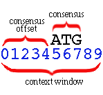
The consensus (e.g., ATG for a start-codon
sensor) is expected at a particular offset from the left of the context
window. This offset is the consensus offset. In the
example
above the consensus offset is 5, and the consensus length
is 3.
The context window has length 10 in this example. These
parameters must be given to the training procedures so they may
correctly parse the training data and observe the positional statistics
relative to the signal consensus.
The simple model types are trained using the train-signal.pl
script. Running the script with no parameters gives you the
following usage statement:
tigrscan/train-signal.pl <model-type> <pos.fasta> <neg.fasta> <filestem> <%train>
     <signal-type> <consensus-offset> <consensus-length> <context-window-length>
     <min-sens> <order> <min-sample-size> <boosting-iterations>
where
     <model-type> is one of {WMM,WAM,WWAM}
     <signal-type> is one of {ATG,TAG,GT,AG,PROMOTER,POLYA}
The parameters are as follows:
<model-type>
|
one of WMM, WAM, WWAM
|
<pos.fasta>
|
one of the multi-FASTA files of positive example
sequences generated by the get-examples.pl script
|
<neg.fasta>
|
one of the multifasta files of negative example
sequences generated by the get-negative-examples-iso.pl script
|
<filestem>
|
filestem for output file -- e.g., "initial-exons"
|
<%train>
|
fraction of the training set to use for
training; zero to one (e.g., use 0.8 to denote 80%); the remainder will
be used for testing
|
<signal-type>
|
one of ATG, TAG, GT, AG, PROMOTER, POLYA
|
<consensus-offset>
|
the number of bases to the left of the consensus
in the model window
|
<consensus-length>
|
the length of the consensus; e.g., 3 for ATG, 2
for GT
|
<context-window-length>
|
length of the model window or weight matrix
|
<min-sens>
|
minimum sensitivity required; e.g. 0.99
indicates that you are willing to miss at most 1% of the true signals
|
<order>
|
Markov order for WAMs and WWAMs; ignored for WMMs
|
<min-sample-size>
|
in WAMs and WWAMs, this is the minimum sample
size required for using n-gram ("n-mer") statistics for a given n-gram
in the Markov chains (otherwise a shorter n-gram is used to obtain
larger sample size).
|
<boosting-iterations>
|
number of times to duplicate the incorrectly
classified training signals and retrain the model with the modified
training set
|
Here are some examples:
train-signal.pl WAM start-codons0-100.fasta
non-start-codons0-100.fasta start-codons0-100 1 ATG 15 3 33 0.98 1 80 0
train-signal.pl WAM stop-codons0-100.fasta
non-stop-codons0-100.fasta stop-codons0-100 1 TAG 0 3 53 0.98 1 80 0
train-signal.pl WAM donors0-100.fasta non-donors0-100.fasta
donors0-100 1 GT 20 2 63 0.98 0 400 6
train-signal.pl WAM acceptors0-100.fasta non-acceptors0-100.fasta
acceptors0-100 1 AG 25 2 43 0.98 0 80 5
|
NOTE: |
 |
|
For your convenience, these
commands can be found in
the train.sh shell script included in the TigrScan
distribution. |
When the <%train>
parameter is less than 1, the signal trainer produces a *.prec-recall
file and a *.scores file. These can be used to
assess the quality of the model. Both files can be graphed with
the xgraph program, which is distributed
with TigrScan.
The *.scores graph will show you how well the scores of the
positive and negative examples separate -- the more they separate, the
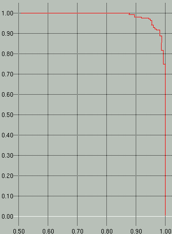
better. The *.prec-recall graph shows a precision vs.
recall (specificity vs. sensitivity) graph, with recall on the y-axis
and precision on the x-axis.
Sample *.scores and *.prec-recall graphs are shown
below. In the scores graph on the left, you can see that the
positive examples (red) separate very nicely from the negative examples
(green). In the graph on the right we see that to attain a
sensitivity (y-axis) of 100% we would have to accept a specificity
(x-axis) of ~88%.
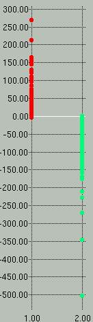
The *.scores graph can be displayed with the
command xgraph -nl -P <filename>, whereas the *.prec-recall
graph can be displayed using the command xgraph <filename>.
The training of an MDD model is performed
similarly. The training script is called train-mdd.pl
and has the following usage statement:
train-mdd.pl <model-type> <pos.fasta> <neg.fasta> <filestem> <% train>
     <signal-type> <consensus-offset> <consensus-length>
     <context-window-length> <min-sens> <order>
     <min-sample-size> <max-depth> <WWAM-wnd-size> <use-pooled-model(0/1)>
The parameters are as described above for the
train-signal.pl script, except as follows:
<model-type>
|
the type of model to be used at the leaves of
the MDD tree
|
<max-depth>
|
maximum depth of the MDD tree
|
<use-pooled-model>
(0 or 1)
|
if this is set to 1, then the MDD tree will be
used to select a leaf model, and then the score from that leaf model
will be averaged with the score from a pooled model -- otherwise, if
set to 0, then only the MDD leaf model will be used
|
See (Burge, 1997) or (Burge and Karlin, 1997) for a description
of MDD.
Step 5. Training content
sensors
Content sensors are models which are used to score the
variable-length regions of a parse. These include:
introns
|
coding exons
|
intergenic segments
|
UTR segments
|
The train-content-sensor program has this
usage statement:
train-content-sensor -g [-o order] [-s MinSampleSize] [-r <null.model>]
                     MC|3P <pos.fasta> <neg.fasta> <output-filestem>
                     <%train> <content-type>
where -e evaluates performance of model using the given negative examples
      -g outputs a precision-recall graph (requires -e)
      -o sets the Markov order for MC, WAM, or 3P
      -r causes the model to use log-odds ratios instead of probabilities
         (the model file is optional; w/o it we use the model's rev. comp.)
      MC = Nth-order Markov chain (1st order by default)
      3P = 3-periodic Nth-order Markov chain
      <%train> = portion of training set to use for training (vs. testing)
                 (example: 0.90 = hold out 10% for testing)
      <content-type> =
         INTRON|INTERGENIC|SINGLE-EXON|INITIAL-EXON|INTERNAL-EXON|
         FINAL-EXONS|THREE-PRIME-UTR|FIVE-PRIME-UTR
The available content models are currently Markov
chains (MC) and three-periodic (inhomogeneous) Markov chains. The
order of these Markov chains is specified with the -o
option.
The -g and -e options cause a *.prec-recall
graph to be produced, as with train-signal.pl. Note,
however,
that this graph is somewhat less meaningful for content sensors than
for signal sensors. In the case of signal sensors, an explicit
cutoff threshold is determined empirically from the precision vs.
recall graph, and this threshold is used to determine which occurrences
of a consensus (e.g., GT or ATG, etc.) will be instantiated as signals
in the gene finder's
dynamic programming algorithm. For content sensors, however, no
such threshold is appled, so the precision vs. recall graph is only
produced to help you evaluate the quality of the model when exploring
the parameter space of the model during training.
Use of the -r option is not recommended at this time.
It is experimental.
The remainder of the parameters and options should be
self-explanatory. Most of them are directly analogous to those
used during the training of the signal sensors.
The following examples show some reasonable parameterizations for each
of the content types:
train-content-sensor -o 5 -s 80 3P initial-exons0-100.fasta
	non-initial-exons0-100.fasta initial-exons0-100 1.0 INITIAL-EXON -g

train-content-sensor -o 5 -s 80 3P final-exons0-100.fasta
	non-final-exons0-100.fasta final-exons0-100 1.0 FINAL-EXON -g

train-content-sensor -o 5 -s 80 3P internal-exons0-100.fasta
	non-internal-exons0-100.fasta internal-exons0-100 1.0 INTERNAL-EXON -g

train-content-sensor -o 5 -s 80 3P single-exons0-100.fasta
	non-single-exons0-100.fasta single-exons0-100 1.0 SINGLE-EXON -g

train-content-sensor -o 5 -s 80 MC introns0-100.fasta
	non-introns0-100.fasta introns0-100 1.0 INTRON -g

train-content-sensor -o 0 -s 80 MC intergenic0-100.fasta
	non-intergenic0-100.fasta intergenic0-100 1.0 INTERGENIC -g

train-content-sensor -o 1 -s 80 MC five-prime-UTR0-100.fasta
	three-prime-UTR0-100.fasta five-prime-UTR0-100 1.0 FIVE-PRIME-UTR -g

train-content-sensor -o 1 -s 80 MC three-prime-UTR0-100.fasta
	five-prime-UTR0-100.fasta three-prime-UTR0-100 1.0 THREE-PRIME-UTR -g
|
NOTE: |
|
|
For your convenience, these
commands can be found in
the train.sh shell script included in the TigrScan
distribution. |
Step 6. Generate
distributions
Exon length distributions
TigrScan uses geometric distributions to model
noncoding segment lengths, but the exon length distributions must be
inferred from the training data. To do this, type:
get-distributions.pl . 5 20
This will create create a *.distr file for each of the
exon types,
for each of the isochores. The parameters to this script are:
output-directory
(or dot, ".")
|
where the *.distr files will be written
|
smoothing-window-size
|
the size of the averaging-windows used for
smoothing the distribution
|
smoothing-iterations
|
the number of times to apply the smoothing
windows
|
The get-distributions.pl script
applies a simple smoothing using a fixed-size, sliding window.
Each point in the distribution is replaced with the average of the
values in the window centered around that point. If you do not
want to apply any smoothing then specify 0 for the second and third
parameters.
You can view a distribution using the xgraph
program via the command:
xgraph <filename>
State transition probabilities
The probabilities of transitioning between particular states in
the GHMM can be estimated from the training data via the following
command:
get-trans-distr.pl iso0-100.gff > trans0-100.txt
This can be done separately for each isochore. The
probabilities in the output file are well-labeled, so you should be
able to modify them if necessary.
Mean noncoding lengths
When you modify the configuration file (below)
you will need to specify the mean lengths of noncoding segments.
For the introns, this can be collected from the training data as
follows:
get-mean-intron-length.pl introns0-100.fasta
For intergenic regions, you have to guess, based on your
estimation of the genome size, the number of genes in the genome, and
the average gene extent (from the start codon to the stop codon,
including introns). A trivial script has been provided to perform
the requisite calculation:
guess-mean-intergenic-length.pl <num-genes>
<gene-length> <genome-size>
For mean UTR lengths you will just have to guess, unless you have
sample UTRs.
Step 7. Modify default
configuration file
When TigrScan is executed, the first thing it does is
to read the isochore definition file (*.iso). Two sample
*.iso files are included in the TigrScan distribution, single.iso
for single-isochore operation, and human.iso, which
illustrates the use of multi-isochore operation.
The human.iso file looks like this:
G+C <= 43% : human0-43.cfg
G+C <= 51% : human43-51.cfg
G+C <= 57% : human51-57.cfg
G+C <= 100% : human57-100.cfg
|
After reading this file and determining the G+C content from the
contig it is to annotate, TigrScan then selects the appropriate
configuration file (*.cfg) and loads the parameters and models
specified in that file. A sample configuration file, tigrscan.cfg,
is included in the TigrScan distribution, and looks like this:
##############################################################
#
# basic configuration file for TigrScan
#
#############################################################

donor-model 		= donors.model
donor-consensus 	= GT
acceptor-model 		= acceptors.model
acceptor-consensus	= AG
start-codon-model	= start-codons.model
start-codon-consensus	= ATG
stop-codon-model	= stop-codons.model
stop-codon-consensus	= TAG|TGA|TAA
polya-model		= polya.model
polya-consensus		= AATAAA|ATTAAA
promoter-model		= TATA.model
promoter-consensus	= TATAAA|TATATA|CATAAA|CATATA
initial-exons		= initial-exons.model
internal-exons		= internal-exons.model
final-exons		= final-exons.model
single-exons		= single-exons.model
initial-exon-lengths	= initial-exons.distr
internal-exon-lengths	= internal-exons.distr
final-exon-lengths	= final-exons.distr
single-exon-lengths	= single-exons.distr
mean-intron-length	= 1294
mean-intergenic-length	= 10000
mean-5'-UTR-length	= 769
mean-3'-UTR-length      = 457
introns			= introns.model
intergenic		= intergenic.model
3'-UTR			= three-prime-utr.model
5'-UTR			= five-prime-utr.model
transition-probabilities = trans0-100.txt
probability-start-in-intron = 0
probability-start-in-intergenic = 1
probability-start-in-5pUTR = 0
probability-start-in-3pUTR = 0
queue-capacity = 1
exon-optimism = 0
intron-optimism = 0
|
Note that any characters occurring after a # on a line
are ignored.
The *.model files are
those which you generated during training of the signal and content
sensors. The *.distr files are those which you
generated for the exon length distributions. The mean intergenic,
exon, and UTR lengths are specified in base pairs. The state
transition probabilities are given in the specified file. The
probability-start-in-* parameters give the probabilities of the
GHMM starting in the given state, and also of ending in the same
state. The exon-optimism and intron-optimism
values are added to the log probabilities for transitioning into an
exon or intron state, respectively. The queue-capacity
value should be set to 1 for normal gene-finding operation -- other
values are useful only when compiling the program with USE_EXPLICIT_GRAPHS
turned on.
The only other parameters shown here are the signal consensus
parameters. If a signal can have more than one consensus, use the
vertical bar (|) to separate them. You can use the get-consensus.pl
script to determine whether any of your training data uses
non-canonical splice sites or start-/stop-codons:
get-consensus.pl 0-100
The observed consensus sequences will be displayed along with their
counts. Obviously, this script must be applied to each isochore.
Step 8. Optimize the
gene finder
There are many things that you can do to try to improve the
accurcy of the gene finder. Several approaches are described
below. You might try any or all of them, in different
combinations, until you achieve the desired level of accuracy.
Pooling exon types
Rather than training a separate model for initial exons, internal
exons, final exons, and single exons, you can pool all the exon types
and train a single exon model. Simply use the cat
command to combine the multi-FASTA and GFF files into a single FASTA
and GFF file, and then train a single model from these as described
earlier. Then, in the configuration file, specify that one model
rather than the separate models.
This might be helpful if you have a very limited amount of training
data.
Modifying signal thresholds
The third line in each signal's *.model file contains
the threshold value which is used decide whether a consensus sequence
should be considered an instance of that signal. You might try
experimenting with different values on this line. Alternatively,
you can retrain your signal sensors with different <min-sens>
(sensitivity) values.
Use different isochore definitions
You might try using different numbers of isochores, different
isochore boundaries, or using no isochores at all (i.e., 0-100%
GC). If you have very little training data, you will probably
reduce the accuracy by using more than one isochore.
Use different types of models
You should try using all of the model types available. For
signal sensors, that currently includes WMMs, WAMs, and WWAMs, as well
as MDD trees. You should not necessarily assume that any one of
these is superior to the others without actually trying it for your
data.
Parameterize your models differently
Consider changing the parameters used during training,
including the Markov orders, the window sizes and consensus offsets,
the minimum sample sizes, the minimum sensitivity, and number of
boosting itereations.
Smooth your length distributions differently
The length distributions might be overly distorted from the
smoothing you have applied. Try using different smoothing
parameters and view the results using xgraph to
check whether the resulting curves look reasonable.
Modify the mean noncoding lengths
Any of the mean noncoding lengths (intron, intergenic, UTR) might
be profitably modified, even those that were observed from the training
data.
Miscellany
A. Invoking the train-signal-sensor program
directly
The train-signal.pl script invokes the train-signal-sensor
program. If you wish to invoke that program directly, its usage
statement is as follows:
train-signal-sensor -g [-o order] [-s MinSampleSize] [-r <null.model>]
                    WMM|WAM|WWAM <pos.fasta> <neg.fasta> <output-filestem>
                    <%train> <signal-type> <consensus-offset> <consensus-length>
                    <min-sensitivity> [-b boosting-threshold]
where -e evaluates performance of model using the given negative examples
      -g outputs a precision-recall graph (requires -e)
      -o sets the Markov order for MC, WAM, or 3P
      -r causes model to use log-odds ratios instead of log-probabilities
         (the model file is optional; w/o it we use the model's rev. comp.)
      WMM = position-specific weight matrix
      WAM = weight array matrix
      WWAM = windowed weight array matrix
      <%train> = portion of training set to use for training (vs. testing)
                 (example: 0.90 = hold out 10% for testing)
      <signal-type> = ATG|TAG|GT|AG|PROMOTER|POLYA
      <min-sensitivity> = (for example) 0.98
Note, however, that the example signals extracted by
the get-examples.pl script contain an extra 80bp on either
side of the signal, which the train-signal.pl script pares
down to include just the specified context window before passing this
sequence to train-signal-sensor. Failing to do this
before calling train-signal-sensor will create problems.
B. Invoking the mdd program directly
The train-mdd.pl script invokes the mdd
program. If you wish to invoke that program directly, its usage
statement is as follows:
mdd <consensus-offset> <consensus-length>
    <model-type> <signal-type> <pos.fasta> <neg.fasta> <out-filestem>
    <min-recall> <%train> [-d max-depth][-s #][-o #][-w #]

     -d = maximum MDD tree depth
     -s = min sample size for Markov chains
     -o = max order for Markov chains
     -w = "windowing" size for WWAM
     -p = incorporate a pooled model
     model types: WMM,WAM,WWAM
     <%train> = portion of training set used for training (vs. testing)
C. The xgraph Program
Included in the TigrScan distribution is a useful tool called xgraph,
written by David Harrison at UC Berkeley. When you unpack the
TigrScan distribution file you will find the file xgraph.tar.gz
in the current directory. Use gunzip and tar -xvf
to unpack this file. You may then try to use the ./xgraph
binary (compiled for Linux), or if this does not work on your system
you can compile the source code.
The following copyright notice can be found in the xgraph
source code, which is included in the TigrScan distribution:
 * Copyright (c) 1988, 1989, Regents of the University of California.
 * All rights reserved.
 *
 * Use and copying of this software and preparation of derivative works
 * based upon this software are permitted.  However, any distribution of
 * this software or derivative works must include the above copyright
 * notice.
References
Burge, C. (1997) Identification of Genes
in Human Genomic DNA. PhD Thesis, Stanford University.
Burge, C. and Karlin, S. (1997)
Prediction of complete gene structures in human genomic DNA. J.
Mol. Biol. 268, 78-94.